
Understanding the Perceptron: How Machines Learn Decision Boundaries
Our mission is to make your business better through technology
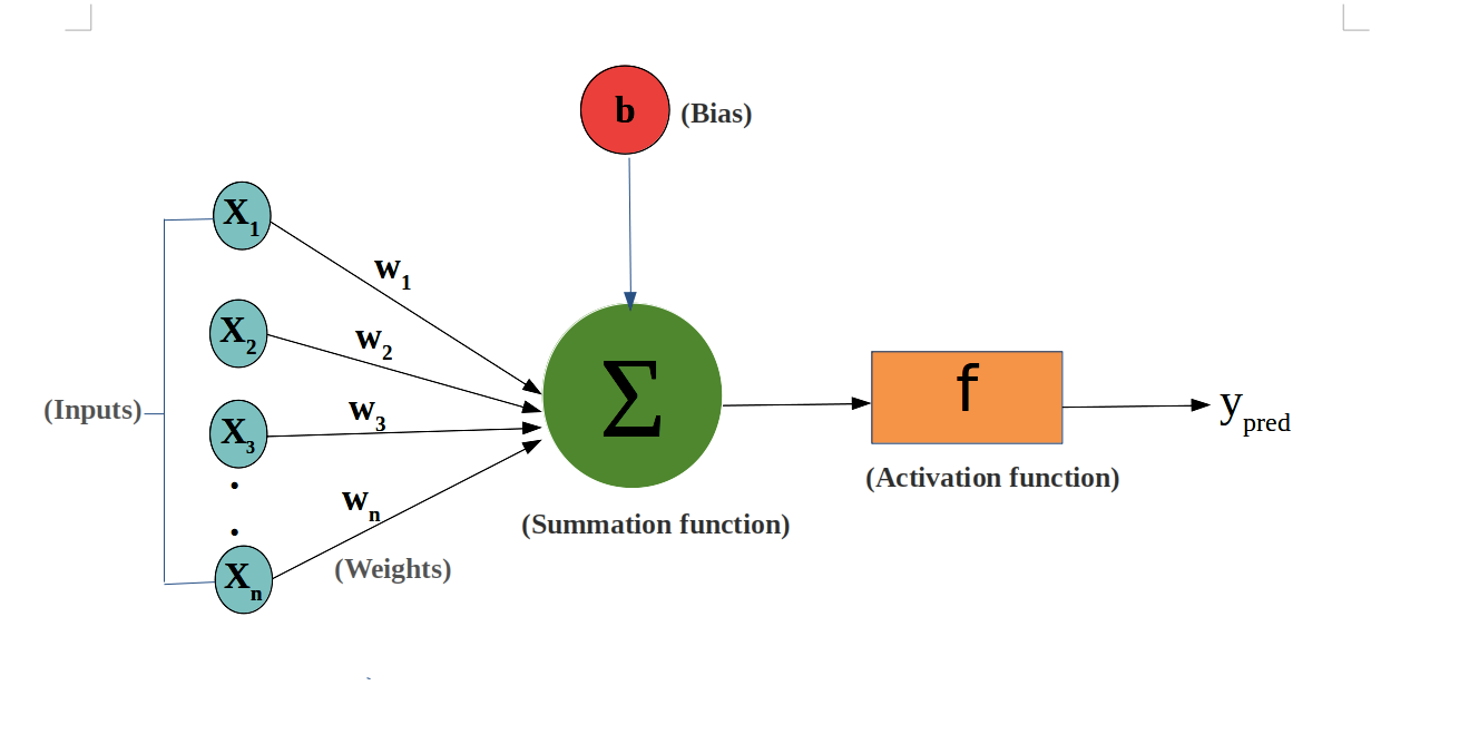
Table of Contents
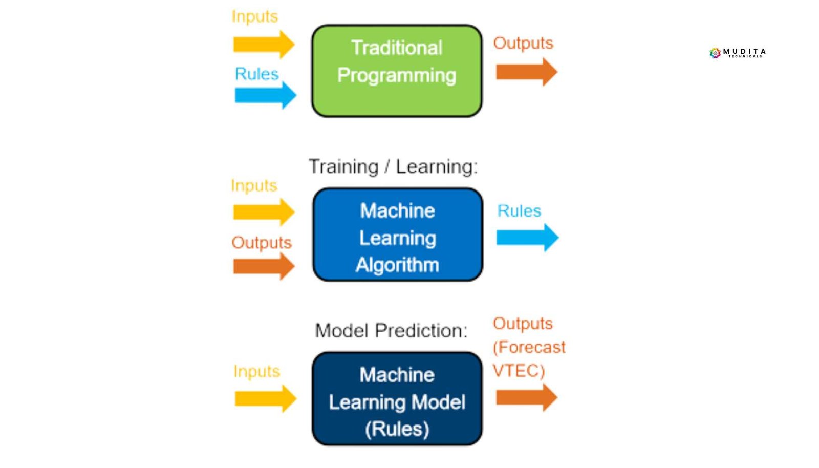
The World Before Machine Learning
Before machine learning existed, computers were unable to learn from data. They could only follow explicitly programmed rules, where every possible condition had to be anticipated and written by a human in advance.
As a result, such systems often failed when they encountered situations that were not covered by predefined logic.
Key limitation:
There was no general mechanism for computers to improve their behavior using examples. This limitation created the need for learning-based approaches.
Why the Perceptron Was Introduced
The perceptron was introduced to answer a fundamental question:
How can a machine learn from data instead of relying on hand-written rules?
It was one of the earliest models capable of adjusting itself automatically based on training examples. This represented a foundational shift toward what we now call machine learning. The idea was proposed by Frank Rosenblatt in the late 1950s.
What Is the Perceptron?
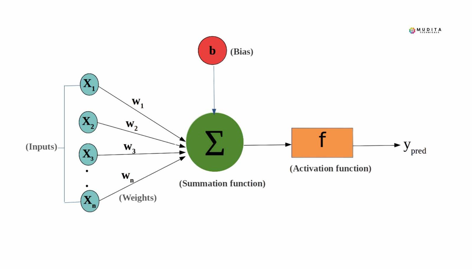
At a high level, a perceptron is a simple computational model inspired by biological neurons. It is designed to make binary decisions, such as yes/no or 0/1. Instead of following explicit rules, the perceptron relies on parameters that can be learned from data.
Inputs: What Information the Model Uses
Inputs, also called features, are the pieces of information provided to the perceptron.
Examples include:
- Email classification: number of links, presence of suspicious words
- House price prediction (simplified): size of the house, number of rooms.
By themselves, inputs do not define a decision. The model must interpret them.
Weights: Learning What Matters
A weight represents the importance of an input feature.
- A high weight indicates that the input has a strong influence on the output.
- A low weight means the influence is weaker.
- A weight of zero effectively ignores the input.
Learning in a perceptron largely consists of adjusting these weights.
Bias: The Baseline Decision
The bias allows the perceptron to make decisions even when all input values are zero. It represents the model’s baseline tendency before observing any input.
Without a bias term, the model would be overly rigid and less capable of learning flexible decision boundaries.
Combining Inputs, Weights, and Bias
To compute a decision, the perceptron:
- Multiplies each input by its corresponding weight.
- Sums the weighted inputs.
- Adds the bias
The result is a weighted sum that serves as the model’s raw decision score.
Activation Function: Making the Final Decision
This weighted sum is passed through an activation function. In a perceptron, this is typically a step function.
- If the result is greater than or equal to zero, the output is 1
- If the result is less than zero, the output is 0
This step converts the raw score into a binary prediction.
What the Perceptron Computes Internally
For a two-dimensional input with features x1 and x2, the perceptron computes:
z=w1x1+w2x2+b
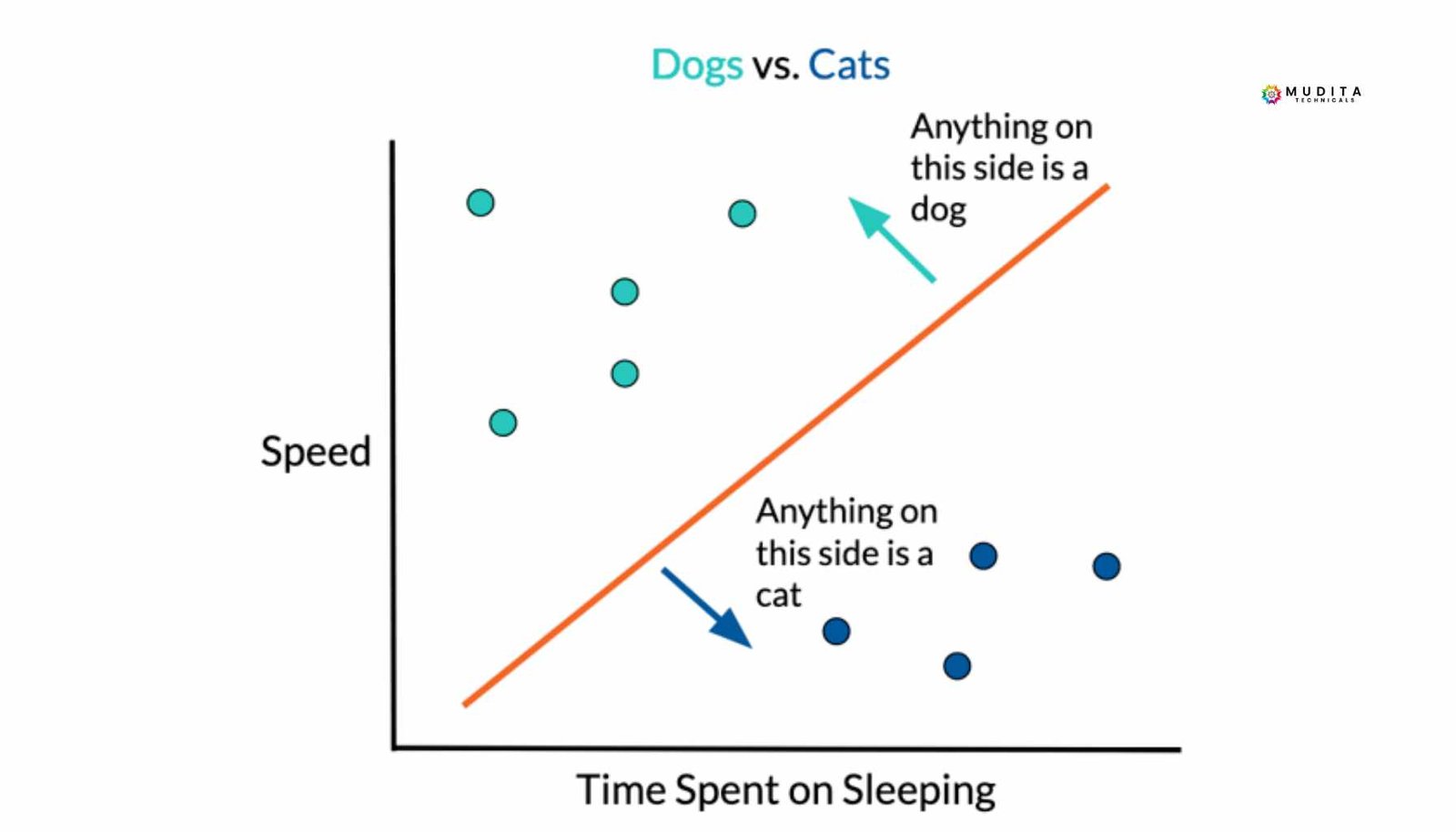
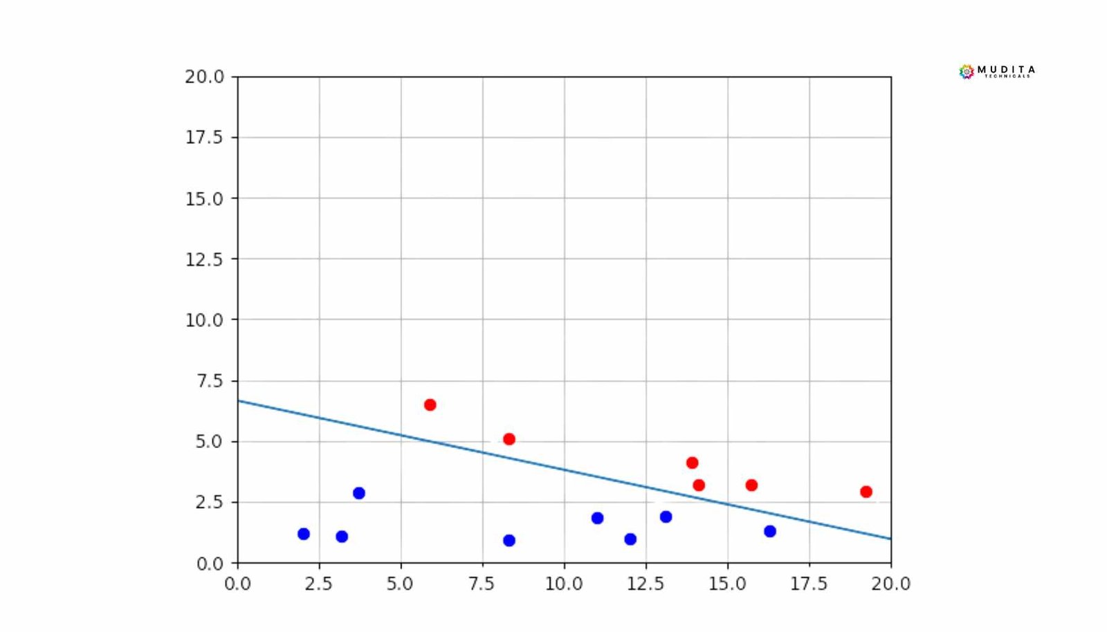
This equation represents a straight line in a two-dimensional feature space. The value z is not the class label; it is a score that indicates which side of the line a point lies on.
The perceptron then applies the activation rule:
- If z>0z > 0z>0, the output is 1
- If z<0z < 0z<0, the output is 0
The line defined by
w1x1+w2x2+b=0
is called the decision boundary.
Points on one side of the boundary are classified as Class 1, while points on the other side are classified as Class 0.
Role of Weights in the Decision Boundary
Weights determine the orientation, or slope, of the decision boundary.
- A larger w1 increases the influence of Feature 1
- A larger w2 increases the influence of Feature 2
Changing the weights rotates the boundary.
Role of Bias in the Decision Boundary
The bias determines the position of the decision boundary.
- A positive bias shifts the boundary in one direction.
- A negative bias shifts it in the opposite direction
Changing the bias moves the boundary without changing its orientation
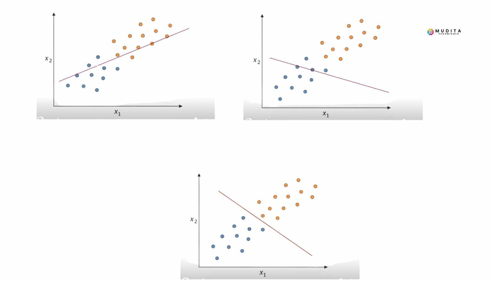
Learning as Boundary Adjustment
During training:
- A data point is misclassified.
- The perceptron updates its weights and bias.
- The decision boundary shifts or rotates.
- Fewer points are misclassified in later iterations
Learning can therefore be understood as the gradual adjustment of the decision boundary to better separate the data..
An Intuitive View of the Perceptron
The perceptron can be thought of as a system that draws a line and declares:
“Everything on this side belongs to Class 1. Everything on the other side belongs to Class 0.”
It then keeps adjusting that line until it best fits the data.
Share this :

Monica Singh is a dynamic professional with expertise in technology, digital growth, and strategic thinking. Passionate about innovation, she focuses on creating impactful solutions, continuous learning, and driving meaningful results through collaboration and modern digital practices.





1 thought on “Understanding the Perceptron: How Machines Learn Decision Boundaries”
Thi is a great article no doubt about it, i just started following you and i enjoy reading this piece. Do you post often ? we have similar post on the german best freelancer platform called https://webdesignfreelancerdeutschland.de/ you can check it out if you want. Thank you